Gmm Model
🧠 Customer Segmentation with Gaussian Mixture Models (GMM) – Practical Guide
In this blog post, we’ll explore Gaussian Mixture Models (GMM) for unsupervised learning, especially for customer segmentation, using a real-world dataset: Mall Customer Segmentation Data.
📦 Dataset Used
The dataset contains demographic and spending data of mall customers:
- Age
- Annual Income
- Spending Score
Source: Kaggle - Mall Customer Segmentation Data
🔧 Step 1: Load and Prepare the Data
1
2
3
4
5
6
7
8
9
10
11
12
13
import pandas as pd
import numpy as np
from sklearn.preprocessing import StandardScaler

# Load dataset
df = pd.read_csv("mall_customers.csv")

# Drop unneeded columns
df = df.drop(['CustomerID', 'Gender'], axis=1)

# Scale the features
scaler = StandardScaler()
X_scaled = scaler.fit_transform(df)
We drop CustomerID and Gender for simplicity and scale the features to give equal weightage.
🤖 Step 2: KMeans vs GMM
Before diving into GMM, we also compare it with KMeans clustering.
1
2
3
4
5
6
7
8
9
10
from sklearn.cluster import KMeans
from sklearn.mixture import GaussianMixture

# KMeans Clustering
kmeans = KMeans(n_clusters=3, random_state=42)
kmeans_labels = kmeans.fit_predict(X_scaled)

# Gaussian Mixture Model
gmm = GaussianMixture(n_components=3, random_state=42)
gmm_labels = gmm.fit_predict(X_scaled)
Unlike KMeans which assigns each point to a cluster hard, GMM uses soft clustering (probability distributions).
📊 Step 3: Visualize Results with PCA
We use PCA to reduce features into 2D for visual clarity:
1
2
3
4
5
6
7
8
9
10
11
from sklearn.decomposition import PCA
import matplotlib.pyplot as plt
import seaborn as sns

pca = PCA(n_components=2)
X_pca = pca.fit_transform(X_scaled)

# Prepare DataFrame for plotting
plot_df = pd.DataFrame(X_pca, columns=['PC1', 'PC2'])
plot_df['KMeans_Cluster'] = kmeans_labels
plot_df['GMM_Cluster'] = gmm_labels
🖼️ KMeans vs GMM Clustering
1
2
3
4
5
6
7
8
9
10
fig, axs = plt.subplots(1, 2, figsize=(14, 6))

sns.scatterplot(data=plot_df, x='PC1', y='PC2', hue='KMeans_Cluster', ax=axs[0], palette='Set2')
axs[0].set_title('KMeans Clustering Results')

sns.scatterplot(data=plot_df, x='PC1', y='PC2', hue='GMM_Cluster', ax=axs[1], palette='Set2')
axs[1].set_title('Gaussian Mixture Model Clustering Results')

plt.tight_layout()
plt.show()
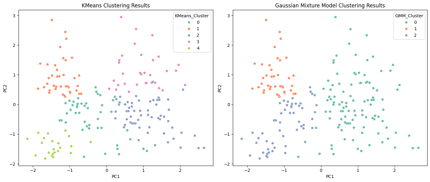
GMM provides more flexible and natural boundaries between clusters, unlike KMeans which assumes spherical shapes.
🤔 Why GMM?
- GMM can model elliptical clusters — better for real-world data.
- Supports soft clustering — gives probability of belonging to each cluster.
- More adaptable than KMeans in non-spherical distributions.
📌 Final Thoughts
Gaussian Mixture Models are powerful for segmentation tasks where boundaries aren’t strictly defined. This makes them ideal for marketing, finance, biology, and more.
💾 Repository + Resources
- Full Code & Dataset: GitHub Repo
- Visuals included
- Feel free to fork and modify!
Follow me for more ML experiments and hands-on tutorials!
Blog by Saddam Hossain — LinkedIn